When you think of "tools for machine learning" then it is likely that you'll think about...
In a lot of machine learning pipelines it can be very beneficial to scale your data before handing it off to a machine learning algorithm. Some algorithms are able to cope with unbalanced columns better than others, but in general it is seen as a good practice to keep this scale in mind. There are a lot of ways that you could do this, but a very popular method is the StandardScaler from scikit-learn. It works by subtracting the mean from every column and dividing by the variation.
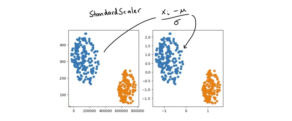
From the outset, this StandardScaler may seem like a very simple thing to implement. After all, you only need to calculate the mean and the standard deviation per column. That implementation, roughly, should just be this:
# At fit time, semi pseudo code
center, variation = {}, {}
for column in dataset.columns:
	center[column] = np.mean(dataset[column])
	variation[column] = np.std(dataset[column])

# At predict time, semi pseudo code
scaled_dataset = dataset.copy()
for column in scaled_dataset.columns:
	mean = center[column]
	stdev = variation[column]
	scaled_dataset[column] = (scaled_dataset[column] - mean) / stdev
It might sound counterintuitive, but the standard scaler inside of scikit-learn does **so much more than this**. It might feel hard to believe at first, but in a lot of ways this code does not reflect reality. That's because a lot of what scikit-learn does on your behalf is invisible. The goal of this blogpost is to go deep here and attempt to demonstrate that the StandardScaler is definately not standard as far as the implementation goes.
Dealing with sparsity
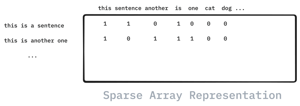
There are a lot of little things that scikit-learn supports under the hood because use-cases can be quite varied. If you are dealing with text, just to name one example, then you are typically dealing with the `CountVectorizer` in scikit-learn to turn the text into a bag of words representation. These representations can represent many thousands for words which is why they are best stored in a sparse representation. That way, you will only need to store the indices of the data that actually contain a word and not waste any memory storing any zeros.
This is all very neat, but what if somebody wants to scale this data? In that case you would not be able to scale the mean of the columns, because that would quickly turn the data into a dense format again. All the zeros that we did not store in the sparse format now become non-zero and the dataset may no longer fit in memory!
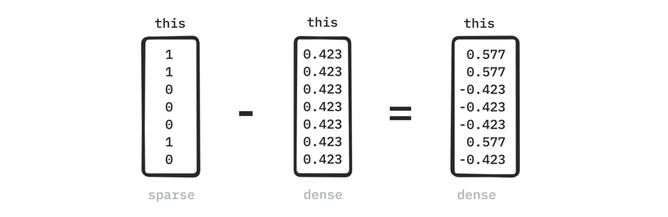
But this is not the case if we arewcc interested in just scaling the variation! In that case we could get away with only updating the non-zero indices! And that's the thing ... if we want to allow for this behavior then we will need to have a standard scaler that knows how to deal with sparse arrays! This is certainly do-able, but it requires the implementation to be more than a simple call to numpy.
Dealing with sample weights
Sparse arrays are just one aspect though. Many scikit-learn models also benefit from the ability to weight subsets of your training data differently. If there is an important subgroup within your customer base or if you want to weight the more recent data more heavily then sample weights are a technique to help steer the pipeline in the right direction.
But that might also imply that you want to keep these sample weights in mind when you scale your training data! So that is a feature that the StandardScaler also supports. If you add the sample weights to your pipeline you can also scale your data according to its values.
If you inspect the API documentation you will notice that the fit method allows for a sample weight to be passed along!

Again, this is not the hardest thing to implement, but it again shows that the implementation needs to cover a few extra concerns.
Dealing with online updates
Everything that we've discussed sofar assumes that we are dealing with a dataset that fits in memory. You just need to call `.fit(X, y)` to train the pipeline, but this does imply that `X` and `y` fit in memory. But what if the dataset is too big?
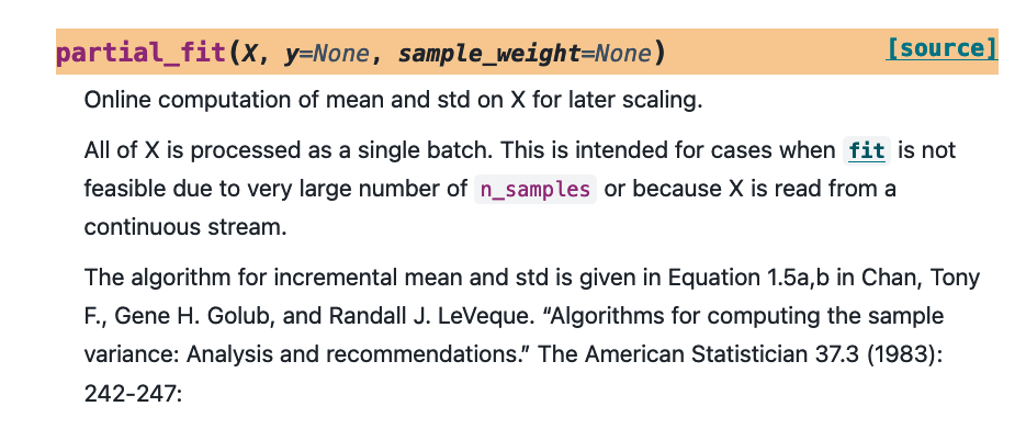
The short answer is that you might train on less data, which is not ideal, or that you train in smaller batches instead. Not every component in scikit-learn has direct support for this but many estimators offer a `.partial_fit()` method. This allows you to feed the estimator one batch of data at a time. As long as the batch of data fits in memory the estimator can learn from it and you can keep on feeding it different subsets over time.
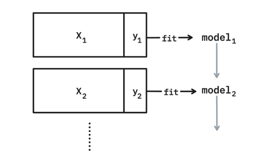
This method of training is not a free lunch. If you are not careful you may suffer from catastrophic forgetting where the most recent batch of training data overshadows the batches that came earlier. But even with these concerns there are plenty of usecases for this technique. The big goal is that everyone can train their machine learning pipelines, even if they are limited by the memory on their machine. So that means that scikit-learn should support this partial fitting technique where-ever possible. And that includes the StandardScaler.
As you can imagine, this makes the implementation a fair bit more involved. You cannot just call `np.mean` and call it a day, you need to store information so that you can continue learning when a new dataset comes in. And because scikit-learn can be used in many different ways it also needs to be robust against users with edge cases. That means that we may be dealing with a small batch of data, and the smallest batch that we can come up with is a batch of just a single datapoint. Put differently: the batch approach needs to be turned into a streaming algorithm that can update when a single new datapoint comes in.
And that's where we will need to talk a little bit about maths. Consider the following formulas for the mean and standard deviation of an array of numbers.
$$ \mu = \sum_i x_i / N $$ $$ \sigma^2 = \sum_i \frac{(x_i - \mu)^2}{N} $$
Turning these into a streaming variant requires us to do a bit of maths, but it is do-able.
For the mean this is relatively easy. Just keep track of how many numbers you've seen sofar as well the sum of all the numbers. When the time comes to emit a mean, you can simply divide the two and you're done. But what about the standard deviation? In the aforementioned formula you can see that in order to calculate the standard deviation we also need the mean.
So how might we deal with this? As luck would have it, we can rewrite the maths some more.
$$ \sigma^2=\frac{\left(\sum_i x_i^2\right)}{N}-\left(\frac{\sum_i x_i}{N}\right)^2 $$
By writing the maths down like this, we can calculate the variance as long as we track some more stats. We just need to keep track of the sum, squared sum and total number of numbers \( N\) that we've seen sofar. That also means that we can write a Python script to track the mean and variance on a stream.
import numpy as np

def calc_mean_var(array):
    n = 0
    sum_xs = 0
    sum_xs2 = 0
    for num in array:
        n += 1
        sum_xs += num
        sum_xs2 += num**2
        yield {
            'n': n,
            'mean': sum_xs / n,
            'std': 0 if n == 1 else np.sqrt(sum_xs2/n - sum_xs*sum_xs/n/n)
        }
You can even give this implementation some simulated data to confirm that it works.
values = np.random.normal(10, 10, 1000)
for i, ex in enumerate(calc_mean_var(values)):
    if i % 100 == 0:
        print(ex)
It takes a while for this loop to converge but it will do so eventually.
{'n': 1,   'mean': 5.173, 'std': 0}
{'n': 101, 'mean': 9.363, 'std': 9.622}
{'n': 201, 'mean': 9.510, 'std': 9.423}
{'n': 301, 'mean': 9.186, 'std': 9.329}
{'n': 401, 'mean': 9.138, 'std': 9.669}
{'n': 501, 'mean': 9.264, 'std': 9.965}
{'n': 601, 'mean': 9.805, 'std': 9.966}
{'n': 701, 'mean': 9.756, 'std': 9.929}
{'n': 801, 'mean': 9.876, 'std': 9.981}
{'n': 901, 'mean': 9.677, 'std': 10.18}
This might sound as a relief. After all, we did the maths and we now have a Python implementation ready to go. So we're done ... right?
Details, details, details!
Unfortunately, this approach will not work. We have to remember that we are dealing with a scaler that needs to deal with axes that are unbalanced. That means, at least potentially, that one axis contains *very* large numbers. And the aforementioned implementation will break because of one single line in the code.
Can you spot it? It is the part where we square the numbers that come in (
sum_xs2 += num**2). Just try it in Python! As an example, let's take a numpy array with very large numbers and square it.# Initialize some large numbers here with small variance
inputs = np.random.normal(10e9, 1, 100)
for i, ex in enumerate(calc_mean_var(values)):
print(ex)
You might get something out that looks like this:
{'n': 1,  'mean': 10000000002.236025,  'std': 0}
{'n': 2,  'mean': 10000000000.730759,  'std': 128.0}
{'n': 3,  'mean': 10000000000.924849,  'std': 0.0}
{'n': 4,  'mean': 10000000000.904922,  'std': 0.0}
{'n': 5,  'mean': 10000000000.835968,  'std': 0.0}
{'n': 6,  'mean': 10000000000.71234,   'std': nan}
{'n': 7,  'mean': 10000000000.45294,   'std': nan}
{'n': 8,  'mean': 10000000000.360819,  'std': nan}
{'n': 9,  'mean': 10000000000.268776,  'std': 0.0}
{'n': 10, 'mean': 10000000000.178272, 'std': 128.0}
The variance can suddenly become zero, not a number or just jump all over the place. You may even see it turn hugely negative! Why?!
It makes a lot of sense once you take a step back and appreciate that numerical algorithms cannot follow pure maths. If a number is too big to fit in the given slot of memory, it will overflow. When you design numeric systems, this is something that always needs to be in the back of your mind. Even if you get the maths perfet you might still end up with numeric inconsistency which can cause havoc to predictive systems. And in this particular case, when you square that huge number, numpy does not have enough bits to store the required number and hence ... it overflows.
Thankfully, one can rewrite the formula even further to make sure that we never square a number in the process. The scikit-learn implementation even refers to it in the docstring, which you can read straight from the documentation page.
If you have a look at the linked article and if you make a base implementation then it might look something like this:
def calc_mean_alternative(array):
    n = 0
    m = None
    v = None
    for num in array:
        n += 1
        prev_m = m
        m = num if m is None else (prev_m + (num - prev_m)/n)
        v = 0 if v is None else (v + (num - prev_m)*(num - m))
        yield {
            'n': n,
            'mean': m,
            'var': 0 if n == 1 else np.sqrt(v/(n - 1))
        }
And when you run this new approach on the same set of large numbers, like so:
values = np.random.normal(10e9, 10, 1000)
for i, ex in enumerate(calc_mean_alternative(values)):
     if i % 100 == 0:
         print(ex)
Then the output looks a lot more sensible, even if it can still take a while for the algorithm to converge properly.
{'n': 1,   'mean': 10000000005.888016, 'var': 0}
{'n': 101, 'mean': 10000000000.339214, 'var': 10.63142545155457}
{'n': 201, 'mean': 9999999999.878897,  'var': 10.901798832837452}
{'n': 301, 'mean': 9999999999.652166,  'var': 10.546990318298718}
{'n': 401, 'mean': 9999999999.926989,  'var': 10.169971560732835}
{'n': 501, 'mean': 10000000000.118559, 'var': 10.148360963235463}
{'n': 601, 'mean': 9999999999.83168,   'var': 10.13434735641984}
{'n': 701, 'mean': 9999999999.876532,  'var': 9.971160210656235}
{'n': 801, 'mean': 9999999999.661884,  'var': 9.977223191586758}
{'n': 901, 'mean': 9999999999.831768,  'var': 9.941820155222036}
And here we see it again. If you want to scale data, there are plenty of edge cases to cover.
The StandardScaler is not standard
When you consider all of this you may experience a renewed appreciation of scikit-learn. There are many edge cases, as well as decades of computer science, that you as an end user do not need to concern yourself with. Scikit-learn does the heavy lifting for you. You don't need to worry about all the relevant numeric details of how to implement these estimators. Instead you can focus on building an appropriate model. That's the beauty of it!
But even if you are not aware of all the details and edge cases, it can still be good to take a moment and to appreciate all the little things that scikit-learn does for you. The StandardScaler is not standard and it would be a shame if we ever took it for granted. There is over a decade of solid work in this library and that has resulted in one of the most reliable machine learning tools on the planet.
And this is just the StandardScaler. Now just try and imagine how much work went into all the other estimators!
ps.
If anything, the appreciation of these little details is one of the main lesson I try to get across with our educational efforts here at probabl. And in particular, the probabl YouTube channel is a big repository for these lessons. You can even find the video version of this blogpost there:
Please check it out if you haven't already!
.png?height=200&name=featured%20image%20badge%20%20(1).png)