You might think that you just landed on yet another blog post on how to "straightforwardly" build a retrieval-augmented generation (RAG) system. Hopefully, it is not the case: we here provide another perspective on the subject, with a special interest in a user problem that we seek to solve rather than focusing solely on the technical and engineering bricks already discussed in other blog posts.

Let's start by outlining our motivations for writing this blog post.

Motivations

A rich documentation and its major drawback

If you are a scikit-learn user, you interact on a daily basis with the scikit-learn documentation website. The scikit-learn documentation is undoubtedly one of the strengths of this open-source project. From the start of the project, particular care is dedicated to documentation writing as much as code writing: the focus is to always provide high-level intuitions and insights on rather technical or theoretical aspects. Thus, the documentation comes in different forms: an application programming interface (API) documentation, an in-depth narrative documentation to present mathematical and methodological aspects, and a gallery of rich usage examples.

However, this rich documentation comes with challenges for scikit-learn users, especially for newcomers: finding the desired information becomes hazardous and rapidly overwhelming. While a true solution to this problem is to curate the documentation as well as possible, providing a tool to search within the documentation is a useful addition. Indeed, all scientific Python packages of the ecosystem (NumPy, SciPy, Pandas, etc.) include a search bar on their website for this purpose.

Search bar: a sub-optimal user experience

This feature is enabled by the Sphinx package that build an index allowing to make some exact search matching. As an example, we could search information related to the random forest classifier in scikit-learn.

While this feature already helps, it fails under those circumstances: (i) it is not robust to typos, (ii) neither to synonyms, and (iii) it is not designed to work with natural language queries. We illustrate this behavior in the following examples:

Prototyping a RAG system under community constraints

In December 2023, we adopted the new pydata-sphinx-theme and were interested in exploring solutions that could alleviate the issues described above. Around the same time, large language models (LLMs) and, more specifically, RAG systems were becoming very popular. Like any hyped technologies, RAG systems were touted as the silver bullet for any information retrieval task at that time. We therefore became interested in prototyping a RAG system to query the scikit-learn documentation, but under constraints imposed by our open-source community work:

• Currently, no personal information from users is collected during queries. Even though this type of information might not be considered sensitive, we do not want to collect and manage any personal user information.
• Our RAG system should only be based on open-source libraries and open-weight models. If we provide our users' data to third-party applications through API, we depend from their terms of service and potential upcoming changes. Open-source libraries and open-weight models allows to be in control over the use of our users' data.
• Being a community-based project, we are limited in terms of financial resources. We should therefore evaluate the cost of offering this search service.

In the remainder of this post, we first explain what a RAG system is. Then, we provide insights into implementing each RAG component. Finally, we discuss the shortcomings of the approach in our particular open-source community context.

Overview of the RAG Pipeline

We expect our user to formulate a natural language query. This query is provided to an LLM model (e.g., Mistral, Llama, GPT-4, etc.), which then provides an answer to the user. In this context, we do not want to provide a back-and-forth conversational agent. This way of using an LLM is also called "zero-shot prompting".

Impossibility of sources checking

In this zero-shot prompting scenario, if the data used to train the model allows it to answer the query, the answer provided by the LLM might already be of reasonable quality. However, obtaining the source backing up the answer is rather impossible. The even worse scenario, in which the LLM was not trained on data containing the answer to the query, will lead to potential hallucinations by the model (note that this can happen even on well trained models sometimes). The situation is even more complex since no sources are provided to double-check the model's answer.

Framed answer with trusted sources

One potential way to alleviate this issue is to add a trusted source of information to our pipeline and this what we usually called RAG. We depict the RAG pipeline in the following manner:

It is very similar to the previous zero-shot prompting scenario presented earlier. However, an additional information retrieval step is added upstream of the query answering process. The goal of this step is to find information related to the query from a trusted source and then request the LLM to answer the user's query using this trusted information (and implicitly its own knowledge). Such a framework potentially limits the hallucinations of the model and provides the user with some sources of information to double-check the answer.

In-depth RAG block analysis

The information retrieval block

While the zero-shot prompting of an LLM is straightforward, the RAG system is adding an information retrieval step. We here discuss a bit more in-depth this topic. Information retrieval is a task that receives significant of attention in both research and industry in the past decades. Let's discuss the principle of the task in our context:

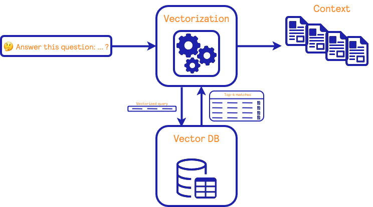
The information retrieval block has two main components: (i) an algorithm to transform natural text into a mathematical vector representation and (ii) a database containing vectors and their corresponding natural text. This database is also capable of finding the most similar vectors to a given query vector.

During the training phase, a source of information containing natural text is used to build a set of vector representations. These vectors are used to populate the database. During the retrieval phase, a user’s query is passed to the algorithm to create a vector representation. Then, the most similar vectors are found in the database, and the corresponding natural texts are returned. These documents are then used as context for the LLM in the RAG system.

Before discussing in more detail the approach to vectorize and find closer vectors algorithms, we first need to have an in-depth look at the definition of a "document" in our context and its practical impacts.

Documents in our context

In our context, we define a document as a part of the documentation that is relevant to answering the user's query. This "part" of documentation is usually referred to as a "chunk". It should be noted that we cannot use the entire documentation page as context of the LLM during the query since this context is limited to a number of tokens by construction. In tutorials that you can find around the internet, a basic strategy of chunking is often advertised and illustrated below:

Garbage chunks in, garbage answer out

Let's take an example where we illustrate shortcomings related to chunking strategies. To this end, let's consider the API documentation of the DummyClassifier that looks like:

This type of documentation can be used to answer questions about parameters, their possible values, their types, etc. For instance, for the DummyClassifier, one could formulate the following question: "What are the values of the strategy parameter in a dummy classifier?".

To this query, an information retrieval system is probably going to get the following chunks.

DummyClassifier	DummyRegressor	SimpleImputer

All chunks match the "strategy" keyword, but unfortunately, this keyword also appears in the documentation of several scikit-learn estimators. With the basic chunking strategy, the chunks do not retain the information related to the estimator. Providing those chunks to the LLM adds a layer of ambiguity and will impact the answer. For instance, using the Mistral 7b model to answer the query with this context results in the following:

"The dummy classifier in scikit-learn does not have a strategy parameter related to generating predictions. Instead, it has parameters like strategry for handling missing values during fitting (with options "mean", "median", "most_frequent", or "constant"). Therefore, there are no specific values for the strategy parameter in a dummy classifier for prediction strategies as mentioned in your query."

Clearly, the answer from the LLM is wrong, but we understand that the model provides a summary of the context. It therefore shows that we need a particular attention when crafting the chunks. For this example, providing the associated estimator name related to the parameter helps at removing the ambiguity.

Chunking strategies

In this section, we describe the three different chunking strategies used for the three different types of documentation.

API documentation

The API documentation is automatically generated from the docstring of the Python classes and functions. We provide an example from the scikit-learn code base that is the docstring of the extract_patches_2d function.

def extract_patches_2d(image, patch_size):
    """Reshape a 2D image into a collection of patches.

    The resulting patches are allocated in a dedicated array.

    Read more in the :ref:`User Guide <image_feature_extraction>`.

    Parameters
    ----------
    image : ndarray of shape (image_height, image_width) or \
        (image_height, image_width, n_channels)
        The original image data. For color images, the last dimension specifies
        the channel: a RGB image would have `n_channels=3`.

    patch_size : tuple of int (patch_height, patch_width)
        The dimensions of one patch.

    Returns
    -------
    patches : array of shape (n_patches, patch_height, patch_width) or \
        (n_patches, patch_height, patch_width, n_channels)
        The collection of patches extracted from the image, where `n_patches`
        is either `max_patches` or the total number of patches that can be
        extracted.

    Examples
    --------
    >>> from sklearn.datasets import load_sample_image
    >>> from sklearn.feature_extraction import image
    >>> # Use the array data from the first image in this dataset:
    >>> one_image = load_sample_image("china.jpg")
    >>> print('Image shape: {}'.format(one_image.shape))
    Image shape: (427, 640, 3)
    >>> patches = image.extract_patches_2d(one_image, (2, 2))
    >>> print('Patches shape: {}'.format(patches.shape))
    Patches shape: (272214, 2, 2, 3)
    """

The docstrings in scikit-learn follow the numpydoc standard to specify parameters, types, examples, etc. The good news is that we can leverage numpydoc, which implements a docstring parser that returns a Python dictionary in which the information from the docstring is structured. We can therefore identify parameters, their associated types and descriptions, etc.

Thus, we create a policy that translates this information into natural language sentences that our LLM knows better how to handle. We provide an example of three chunks automatically generated from the docstring of extract_2d_patches:

For each chunk, we add the associated Python module or class to solve the problem of ambiguity that we earlier show.

Example documentation

The example gallery in scikit-learn leverages another Python package: sphinx-gallery. Similarly to the API documentation, we leverage the example scraper from sphinx-gallery. We have two types of examples in scikit-learn: some simple usage examples and some tutorial examples.

Simple usage example	Tutorial-like example

The simple usage examples (left figure) are composed of a title and a relatively short description followed by a code snippet that usually generates the material discussed in the description. Tutorial-like examples (right figure) are more involved: they are organized into sections where text blocks and code blocks are interlaced.

We therefore use different strategies to create the chunks. For the usage examples, we create one block for the text and one block for the code. Then, we chunk each block independently. For the tutorial-like examples, we first detect the sections in the tutorial, containing both text and code. Since the text and the code within a section are usually related, we do not split them and only chunk this entire block.

User guide documentation

Finally, we have the user guide documentation. For this type of documentation, we use the naive approach for chunking. Since we are interested in a prototype only, this is a good first approximation. We could improve the chunking strategy here by chunking by sections only and making sure that each chunk starts by recalling the table of contents to provide more context.

Information retrieval search

Up to now, we mainly focus on the data that we want to use as context for our LLM. In this section, we go into more detail regarding the approach used to find relevant documents to use as context for our LLM. As previously mentioned, information retrieval is a task that has received a lot of attention in both research and industry. As a short summary, the current state-of-the-art can be split into two approaches: a classical approach based on term frequencies and a machine-learning approach based on neural networks. The following survey by Guo et al. provides an in-depth report of the current state-of-the-art. Here, we briefly present the approaches that we use.

Classical term-based approach

In the classical term-based approach, the idea boils down to computing the frequency of words within a document. Documents belonging to the same topic are expected to have similar term frequencies. A popular concept in this area is known as TF-IDF term weighting, and a retrieval method leveraging this concept to find related documents is BM25. Below, we depict the procedure used to find similar documents using this algorithm.

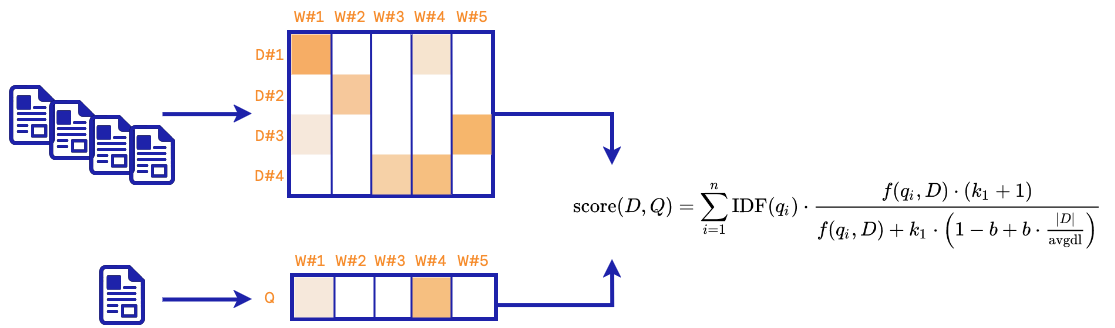
In the training phase, a sparse matrix is created based on the term frequencies of the data collected from the documentation chunks. During the retrieval phase, the query is vectorized using the same term-frequencies strategy, and a score between this vector and each document vector is computed as defined above. The top-k documents are selected and should be the most related to the query.

The BM25 approach, as described here, does not necessarily grasp the semantics in documents or queries. Several methods have been developed to improve the term-based approach in this direction, such as query or document expansions or term dependencies. Here, we do not use any of these approaches and instead combined the BM25 with a neural network approach.

Neural network-based approach

Here, we use a pre-trained Sentence-BERT model. These types of models are intended to learn about semantics.

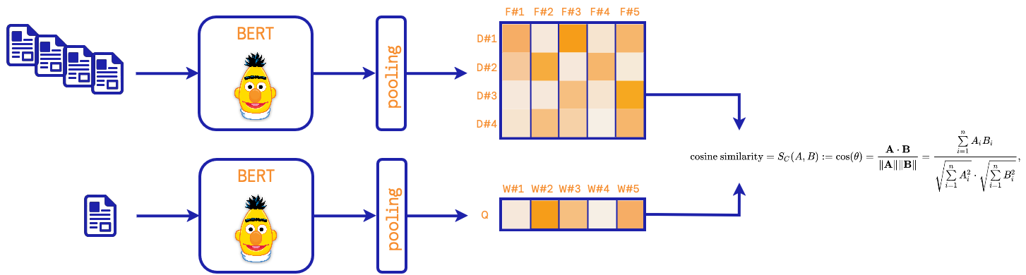
During the training of the model, a BERT model associated with a pooling stage is tuned on pairs of similar/unrelated documents. The pooling strategies and the loss function are part of the implementation details of each model. One consequence of this procedure is that the neural network grasps the semantics behind the documents. At the retrieval stage, a query is then embedded via the BERT model and pooled, and the distance with the trained documents is computed. The top-k documents are found via an approximate nearest neighbor algorithm.

With this approach, it should therefore be noted that we need to select a pre-trained model to embed the documents.

Retrievers in practice

In our prototype, we use both approaches and create different models for different types of documentation. We therefore have three term-based models and three neural network-based models. Once we find the top-k documents via each model, we need to order them from the most relevant to the least relevant.

Documents re-ranking

To re-rank the documents found by the different models, we use a cross-encoder model. The principle is depicted as follows:

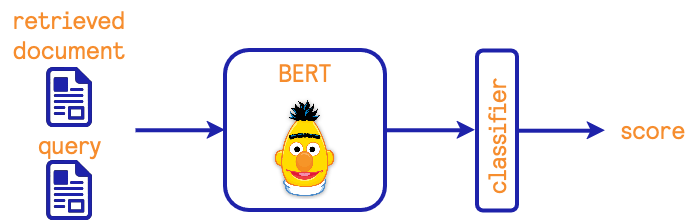
The idea is to provide the user's query and a retrieved document and embed them with a BERT model. The output vector of the BERT model is used by a classifier that provides a similarity score used to re-rank the documents.

The cherry on the top: synthesis with a LLM

Once we retrieve the information helping at answering the user's query, we are ready to request a synthesis from the LLM. While a lot of work is dedicated at crafting the best prompt, here we only created a simple prompt:

 prompt = (
    "[INST] You are a scikit-learn expert that should be able to answer"
    " machine-learning question.\n\nAnswer to the query below using the"
    " additional provided content. The additional content is composed of"
    " the HTML link to the source and the extracted contextual"
    " information.\n\nBe succinct.\n\n"
    "Make sure to use backticks whenever you refer to class, function, "
    "method, or name that contains underscores.\n\n"
    f"query: {query}\n\n{context_query} [/INST]."
)

The library stack for our RAG

In this section, we summarize the different libraries and models that we use to implement our RAG system. We can depict it as follows:

Let's provide a couple of details for each block in this diagram:

• We use our own implementation of the BM25 algorithm
• The bi-encoder and cross-encoder are implemented in the SBERT library. For the bi-encoder model, we use the large version of the General Text Embeddings (gte-large). This model has shown good performance on general retrieval tasks. For the cross-encoder, we use the ms-marco-MiniLM-L-6-v2 model. This model was trained to solve query on the Bing engine.
• The approximate nearest neighbor algorithm uses the FAISS library.
• For the LLM, we use the quantized version of the Mistral 7b v0.2 model. We interface it with the llama-cpp-python library.
• As a chat front-end, we modify the llama.web project to have a minimal interface.

Here, some of the choices are motivated by the following factors:

• The availability and ease of installing a given library.
• For models, the availability of the weights under a permissive license.
• To implement a solution with the minimum number of dependencies and avoid nested or wrapped code by other libraries.

Under other constraints, some of the choices above could be switched to more trendy or more performant libraries or models. We only intend to provide a prototype solution to explore the capacity of a RAG for querying the scikit-learn documentation.

ragger-duck: our reproducible proof-of-concept

While developing this prototype, we wanted to make it fully reproducible. All orchestration of the libraries was consolidated into a GitHub repository called ragger-duck.

The instructions to train and launch the front-end can be found here.

Regarding the concepts that we presented earlier, you can find:

• the script to train the retrievers in this file.
• the application code that loads the encoders, cross-encoder, and the LLM in this file.

The different classes used are documented in the API documentation of ragger-duck.

Final words on shortcomings

Hard to evaluate and fine-tune

While pre-trained models offer the possibility to quickly prototype such a RAG system without a bottleneck regarding the training phase, the cost is moved to the evaluation and fine-tuning stages.

In our context, since we added a constraint of not collecting data, we are not capable of evaluating our RAG or fine-tuning any of the components (retrieval models). Some resources on the internet argue to use other LLMs to evaluate answers provided by a RAG or, as an extension, use those LLMs to create datasets on which to tune the RAG components (e.g., using LoRA). In my humble opinion, those approaches are not methodologically sounding nor correct. Usually, those external LLMs used to evaluate or create datasets are larger and more powerful models. In this context, it is considered that those powerful LLMs provide the gold standard, but there is no reason for it; those LLMs are also known to hallucinate as well.

The only viable action here would be to have an opt-in mechanism for users to send us their search queries and satisfaction regarding the system's answers. This would be an interesting experiment to carry out.

A costly bot?

Finally, there is the question regarding the deployment of this system in production to serve users. First, we can have a look at this cost analysis by AnyScale: the average cost of a request with a similar system as described here is estimated at $0.0003. In the context of scikit-learn, we have around 1 million users checking the documentation per month. If each user starts to make 10 requests a month, then the total cost will be around $3,000 a month. Using a more powerful model would also increase the price. Having a quick look at a cloud provider like Scaleway, the monthly price of a machine with 8 GPUs is around $5,000. Such resources might be required to offer a good user service. It provides a rough estimate of the price of deploying such a system for the community. In terms of financing this service, it would be tricky for the open-source community to finance such an effort. So this is something to keep in mind before envisaging deploying such a solution.

Additional content

This work was presented in PyConDE & PyData Berlin 2024 conference and you can find the videos here.